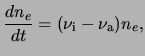
The effect of vertical tropospheric lightning currents on the electron
population at altitudes up to 100 km is modeled in this dissertation with a
finite-difference time domain calculation in cylindrical coordinates,
adapted from that used by Veronis et al. [1999]. The model solves
Maxwell's equations around a vertical symmetry axis, solving for the
vertical and radial electric field, azimuthal magnetic
field, electron density, and ion and electron conduction
currents. The Earth's magnetic field is neglected, as
justified in Figure 1.1 for altitudes up to ![]() 95 km.
Optical emissions are calculated from the electron density and the net
electric field, and instrumental response to the emissions is calculated for a given
geometry and field-of-view.
95 km.
Optical emissions are calculated from the electron density and the net
electric field, and instrumental response to the emissions is calculated for a given
geometry and field-of-view.
These calculations are carried out in three steps. The electron
density
![]() and electric field
and electric field ![]() are calculated as a function
of time and space in the cylindrical geometry. Next, the volume
optical emission rates are calculated from
are calculated as a function
of time and space in the cylindrical geometry. Next, the volume
optical emission rates are calculated from
![]() and
and ![]() in the
same geometry. Finally, the optical signal seen from a chosen vantage
point is calculated using three dimensional geometry. The curvature
of the Earth is taken into account only in this last step; however,
the resulting inaccuracy is small for radial distances
in the
same geometry. Finally, the optical signal seen from a chosen vantage
point is calculated using three dimensional geometry. The curvature
of the Earth is taken into account only in this last step; however,
the resulting inaccuracy is small for radial distances ![]()
![]() 300 km in the
cylindrical geometry.
300 km in the
cylindrical geometry.
A cloud-to-ground lightning return stroke (CG) is modeled by imposing
a current between the ground and a spherical gaussian charge
distribution at 10 km altitude. For lightning currents of
![]() 30
30 ![]() s duration, mesospheric electric fields are dominated by
those of the lightning electromagnetic pulse (EMP), while for
s duration, mesospheric electric fields are dominated by
those of the lightning electromagnetic pulse (EMP), while for
![]() 500
500 ![]() s currents, radiation
effects are negligible and the
quasielectrostatic (QE) field dominates. Both EMP and QE fields are
inherently accounted for in this fully electromagnetic model
[Veronis et al., 1999].
s currents, radiation
effects are negligible and the
quasielectrostatic (QE) field dominates. Both EMP and QE fields are
inherently accounted for in this fully electromagnetic model
[Veronis et al., 1999].
The initial conditions of ![]()
![]() 0,
0,
![]()
![]() 0 allow
0 allow ![]() not to
be recorded explicitly in the calculation. Instead, all changes to
the charge density are accounted for implicitly by the displacement
current, and the resulting fields are fully in accord with Maxwell's
equations, including contributions to the current density
not to
be recorded explicitly in the calculation. Instead, all changes to
the charge density are accounted for implicitly by the displacement
current, and the resulting fields are fully in accord with Maxwell's
equations, including contributions to the current density ![]() from both electrons and ambient (not modified) ion conductivity.
from both electrons and ambient (not modified) ion conductivity.
However, this model is not faithful to the Boltzmann equation
(1.6). The
![]() term, which
accounts for diffusion, is ignored, as is the vector velocity
dependence of the distribution function
term, which
accounts for diffusion, is ignored, as is the vector velocity
dependence of the distribution function ![]() . The effect of the total
electric field
. The effect of the total
electric field
![]() along with all inelastic
collisions is accounted for only through the
swarm parameters for mobility, attachment, and ionization rates. As a
result, changes to the explicitly calculated
along with all inelastic
collisions is accounted for only through the
swarm parameters for mobility, attachment, and ionization rates. As a
result, changes to the explicitly calculated ![]() result from
ionization and attachment, but not from the relatively small
contribution of
result from
ionization and attachment, but not from the relatively small
contribution of
![]() . Nevertheless, ``space charge''
effects on the electric field are accounted for via equation (1.3)
and are evident in the results shown below.
. Nevertheless, ``space charge''
effects on the electric field are accounted for via equation (1.3)
and are evident in the results shown below.
Even more than this absence of fluid (electron transport) properties,
the primary feature which renders the model used here incapable of
reproducing streamer behavior is the
impracticality of numerical solutions with extremely high spatial
resolution. The huge
conductivity gradients
which intensify the electric field at the head of a streamer must be
resolved (and managed in a numerically stable way) in order to produce
a ``self-propagating'' discharge [Pasko et al., 1998a; Dhali and Williams, 1985]. While
this can be done for modeling streamer development at a given altitude
and for a given externally applied initial electric field
[Pasko et al., 1998a], it is impractical to model simultaneously the full temporal
and spatial development of the QE field over the full mesospheric
altitude range. Our
model also does not account for a wide variety of inelastic processes,
such as photoionization, which can play a role in creating free
electrons ahead of a streamer and which become important for the
distribution function at the high values of
![]() in a
streamer head. While ambipolar diffusion is not accounted for in the
current densities used here, it has been shown to be a negligible
consideration even in streamers [Dhali and Williams, 1985], as
compared with the electrostatic effects of unbalanced charge.
in a
streamer head. While ambipolar diffusion is not accounted for in the
current densities used here, it has been shown to be a negligible
consideration even in streamers [Dhali and Williams, 1985], as
compared with the electrostatic effects of unbalanced charge.
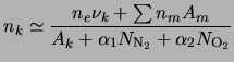
Sections 2.4.1, 2.4.2, and 2.4.3 give the numeric values of various coefficients and cross sections used to account for elastic and inelastic collision processes and to calculate optical emissions in the model. The ionization and attachment coefficients and the rates of molecular excitation responsible for optical emissions have been updated from those used by Veronis et al. [1999], and are based on the compilations and calculations of Pasko et al. [1999a].
Aside from those involving sources and losses of free electrons, all
changes to the electron distribution function are accounted for in the
model by changes to the electron mobility. We use the form
of
![]() provided by Pasko et al. [1997b], which is a polynomial fit to experimental data.
Pasko et al. [1997b] provide references to the experimental data, as
well as a comparison with kinetic calculations.
provided by Pasko et al. [1997b], which is a polynomial fit to experimental data.
Pasko et al. [1997b] provide references to the experimental data, as
well as a comparison with kinetic calculations.
The electron conductivity follows from the
mobility and electron density as
![]() . Conduction
current in the model is calculated using both electron and ambient ion
conductivity [Pasko et al., 1997b].
. Conduction
current in the model is calculated using both electron and ambient ion
conductivity [Pasko et al., 1997b].
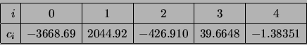
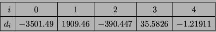
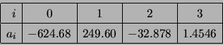
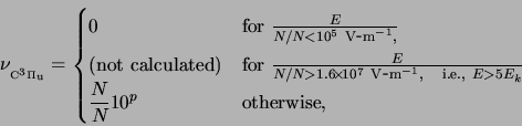
Changes in electron density due to electron impact ionization and dissociative attachment are calculated using
![$\displaystyle p=\sum_{i=0}^{3}a_i\left[
\log_{10}\left( \frac{E}{({\rm 1 \ensuremath{{\rm V\hbox{-}m}^{-1}}\xspace })}\frac{1}{N/N_} \right)
\right]^i$](img184.png)
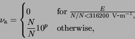
where
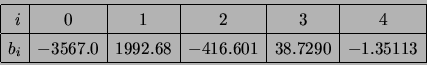
![$\displaystyle p=\sum_{i=0}^{4}b_i\left[
\log_{10}\left( \frac{E}{({\rm 1 \ensuremath{{\rm V\hbox{-}m}^{-1}}\xspace })}\frac{1}{N/N_} \right)
\right]^i$](img189.png)
![\includegraphics[]{figures/ionisationRate.eps}](img194.png) |
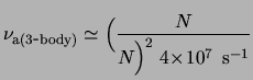
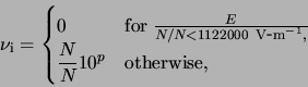
For small electric fields, the three-body attachment process dominates attachment (Section 1.3), and
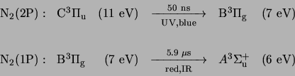
Optical emissions are calculated only from two molecular bands of
neutral N![]() which are expected to dominate the instrument responses
of our photometers (Taranenko et al. [1992] and
Section 3.3). These optical bands are known as the
first positive (1P) and second positive (2P) bands and they result
from transitions between electronic states of N
which are expected to dominate the instrument responses
of our photometers (Taranenko et al. [1992] and
Section 3.3). These optical bands are known as the
first positive (1P) and second positive (2P) bands and they result
from transitions between electronic states of N![]() which have the
following designations and threshold energies:
which have the
following designations and threshold energies:
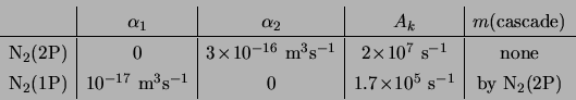
The excitation, quenching, and
cascading processes involved in emission in these bands are discussed
by Pasko et al. [1997b]. We make use of the fact that the lifetimes of
the states
![]() and
and
![]() , given in (2.17), are
fast compared with the variations in electric field and with the
thermal relaxation time
, given in (2.17), are
fast compared with the variations in electric field and with the
thermal relaxation time
![]() of the distribution
function. This fact justifies the assumption that instantaneously the
population
of the distribution
function. This fact justifies the assumption that instantaneously the
population ![]() of the excited state
of the excited state ![]() is constant:
is constant:
![]() , where
, where ![]() corresponds to
corresponds to
![]() or
or
![]() .
The population and depopulation terms for excited state
.
The population and depopulation terms for excited state ![]() are [Sipler and Biondi, 1972]:
are [Sipler and Biondi, 1972]:
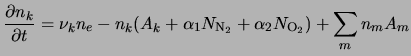
The stationary condition mentioned above gives
The values of the excitation coefficient ![]() were calculated
according to the following polynomial fits [Pasko et al., 1999a]:
were calculated
according to the following polynomial fits [Pasko et al., 1999a]:
![$\displaystyle p=\sum_{i=0}^{4}c_i\left[
\log_{10}\left( \frac{E}{({\rm 1 \ensuremath{{\rm V\hbox{-}m}^{-1}}\xspace })}\frac{1}{N/N_} \right)
\right]^i$](img213.png)