In the mesosphere and the ![]() region of the
ionosphere the properties of the upper atmosphere begin their
transition from those of a neutral gas to a those of a weakly ionized plasma,
as the plasma frequency becomes significant compared with the
effective electron-neutral collision
frequency. This region has also sometimes been called the
``ignorosphere'' because of its inaccessibility to in
situ measurements by either high-altitude aircraft or orbiting
spacecraft, or to remote sensing by ground-based radar or top-side
sounding. Use of sounding rockets, optical remote sensing through
lidar or the photometric and imaging techniques described in this
work, and VLF radio studies lend themselves to investigations of these
awkward altitudes characterized by their relatively low
(
region of the
ionosphere the properties of the upper atmosphere begin their
transition from those of a neutral gas to a those of a weakly ionized plasma,
as the plasma frequency becomes significant compared with the
effective electron-neutral collision
frequency. This region has also sometimes been called the
``ignorosphere'' because of its inaccessibility to in
situ measurements by either high-altitude aircraft or orbiting
spacecraft, or to remote sensing by ground-based radar or top-side
sounding. Use of sounding rockets, optical remote sensing through
lidar or the photometric and imaging techniques described in this
work, and VLF radio studies lend themselves to investigations of these
awkward altitudes characterized by their relatively low
(![]()
![]() cm
cm![]() ) electron densities.
) electron densities.
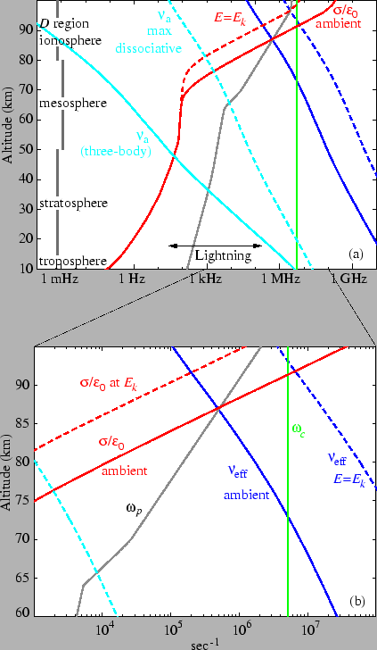
Figure 1.1 compares frequencies and rates of some physical
processes in the lower
ionosphere. The vertical green line shows ![]() , the electron
cyclotron frequency in the Earth's magnetic field.
At 75 to 80 km, the nighttime electron density is similar to that of
the solar wind at 1 AU. In great contrast to solar wind plasma,
however, for altitudes up to
, the electron
cyclotron frequency in the Earth's magnetic field.
At 75 to 80 km, the nighttime electron density is similar to that of
the solar wind at 1 AU. In great contrast to solar wind plasma,
however, for altitudes up to ![]() 70 km under ambient nighttime
conditions, and up to 90 km under an applied electric field near the
breakdown threshold (discussed below in Section 2.1), the
effective collision frequency
70 km under ambient nighttime
conditions, and up to 90 km under an applied electric field near the
breakdown threshold (discussed below in Section 2.1), the
effective collision frequency
![]() for electrons is large compared to the cyclotron
frequency. At night the
electron number density is only 10
for electrons is large compared to the cyclotron
frequency. At night the
electron number density is only 10![]() times the neutral density at 70 km
and
times the neutral density at 70 km
and ![]()
![]() times at 90 km, and on timescales greater than
10
times at 90 km, and on timescales greater than
10 ![]() s, the electrons are in thermal equilibrium with the neutrals,
which are typically at
s, the electrons are in thermal equilibrium with the neutrals,
which are typically at ![]() 300 K. This region may thus be described as a cold,
collisional, weakly ionized electron plasma.
300 K. This region may thus be described as a cold,
collisional, weakly ionized electron plasma.
Representative values of the nighttime electron
density1.1 (
![]() )
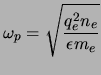
have been used in Figure 1.1. Shown in gray is the electron
plasma frequency,
)
have been used in Figure 1.1. Shown in gray is the electron
plasma frequency,
There are at least three different mechanisms by which thundercloud
charge configurations may impose electric fields on the upper
atmosphere. Thundercloud charging as a result of convective charge
separation occurs on time scales of ![]() 100 s. (Research into the
mechanisms of charge separation and into the nature of charge
configurations in thunderstorms has been ongoing for decades.)
Secondly, sudden and large changes in electrical currents may radiate
electromagnetic fields in all directions. A primary example of such
strongly radiating processes, at least in the frequency range of
interest here, is the return stroke of cloud-to-ground lightning,
whose radiation spectrum peaks with period 50 to 100
100 s. (Research into the
mechanisms of charge separation and into the nature of charge
configurations in thunderstorms has been ongoing for decades.)
Secondly, sudden and large changes in electrical currents may radiate
electromagnetic fields in all directions. A primary example of such
strongly radiating processes, at least in the frequency range of
interest here, is the return stroke of cloud-to-ground lightning,
whose radiation spectrum peaks with period 50 to 100 ![]() s. Third,
continuing currents flowing to ground through return stroke
channels may redistribute large quantities of charge on time scales of
s. Third,
continuing currents flowing to ground through return stroke
channels may redistribute large quantities of charge on time scales of ![]() 0.5 ms
to
0.5 ms
to ![]() 100 ms.
100 ms.
The low-frequency conductivity of the atmosphere
determines whether the electric field
due to these charge configuration changes in thunderstorms can penetrate
to high altitudes. In the absence of significant magnetic fields
(
![]() ), equation (1.3) along with the
constitutive relation
), equation (1.3) along with the
constitutive relation
![]() becomes
becomes
From these simple considerations, some important phenomenological classifications of upper-atmospheric discharges can be presaged. Electric fields due to growing thundercloud charge configurations, which may involve charge centers of hundreds of coulombs [Marshall et al., 1996] but which accumulate over time scales of many tens of seconds, do not affect altitudes much above the troposphere. Space charge developed by currents flowing in accordance with equation (1.8) screen these fields from the thin upper atmosphere. In close vicinity to the tops of thunderclouds, however, such fields are thought to initiate upward streamer-like discharges which can propagate into the stratosphere; these have been denoted blue jets and blue starters [Pasko et al., 1996a; Wescott et al., 1995].
When these same thundercloud charge accumulations are partially
neutralized or redistributed by lightning return strokes and their
continuing currents on much faster timescales than those on which the
charges are built up, the effects penetrate to much higher regions of
the atmosphere. Because of the space charge that builds up in
conjunction with thundercloud charge separation, the upper atmosphere
sees an increase in electric field as a result of any sudden
redistribution of charge, even if the new configuration causes reduced
electric fields in the troposphere. For instance, a large positive
cloud-to-ground return stroke may drain an extensive positive charge
region of ![]() 100 C to the conducting Earth over 1 ms. On short time
scales in the mesosphere, this is entirely equivalent to placing a
negative charge of identical magnitude in the thundercloud.
Considering the electric relaxation rates in Figure 1.1, a
new charge configuration in the troposphere is effective in
allowing the penetration of electric fields up to 85 km if the change
occurs faster than
100 C to the conducting Earth over 1 ms. On short time
scales in the mesosphere, this is entirely equivalent to placing a
negative charge of identical magnitude in the thundercloud.
Considering the electric relaxation rates in Figure 1.1, a
new charge configuration in the troposphere is effective in
allowing the penetration of electric fields up to 85 km if the change
occurs faster than ![]() 1 ms, but only to 70 km if the change occurs
on timescales on the order of
1 ms, but only to 70 km if the change occurs
on timescales on the order of ![]() 10 ms. This principle has
been used in many theoretical studies of sprites
(Section 2.3).
10 ms. This principle has
been used in many theoretical studies of sprites
(Section 2.3).
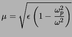
On even faster timescales, radiated electromagnetic fields at VLF
frequencies may penetrate to a height1.2 roughly determined by a
comparison of their frequency with the time scale
![]() . As discussed above, the electromagnetic pulse from
lightning is largely reflected in the
. As discussed above, the electromagnetic pulse from
lightning is largely reflected in the ![]() region, but the
penetration of these fields above the reflection height results, due to
the finite conductivity, in heating of the electron population
(Section 2.1.5).
For strong radiated fields, this energy deposition can produce the
phenomenon known as elves.
region, but the
penetration of these fields above the reflection height results, due to
the finite conductivity, in heating of the electron population
(Section 2.1.5).
For strong radiated fields, this energy deposition can produce the
phenomenon known as elves.
An important complication to the conclusions above results from the
fact that the conductivity itself may
change under an applied electric field. The isotropic conductivity due
to electrons alone is
![]() , and the electron mobility
, and the electron mobility
![]() in turn is a decreasing function of the electric field. The
application of an electric field heats the electron population
(Section 2.1) and increases the
collision frequency
in turn is a decreasing function of the electric field. The
application of an electric field heats the electron population
(Section 2.1) and increases the
collision frequency
![]() , as
shown in Figure 1.1 for a representative electric field
value,
, as
shown in Figure 1.1 for a representative electric field
value,
![]() . Enhanced values of
. Enhanced values of
![]() in turn lead to the decrease
of the mobility and thus the conductivity (Figure 1.1), thus
allowing better penetration of transient electric fields to higher
altitudes.
in turn lead to the decrease
of the mobility and thus the conductivity (Figure 1.1), thus
allowing better penetration of transient electric fields to higher
altitudes.
On the other hand, the electric field can also lead to the
modification of the electron density
![]() through impact
ionization of the neutrals by accelerated electrons and through the
enhancement of electron attachment to neutrals. For example, if
through impact
ionization of the neutrals by accelerated electrons and through the
enhancement of electron attachment to neutrals. For example, if
![]()
![]()
![]() then
then
![]() increases, leading to enhanced conductivity and
reversing the effect of heating described above. Ionization and
heating effects both turn out to be of key importance in sprites and
elves, hence the need arises for detailed modeling to account
self-consistently for the nonlinear effect of an intense and varying
electric field. Such modeling has now been carried out by several
groups, as mentioned in Sections
2.2 and 2.3, and an
electromagnetic model which accounts for these processes is described
in Section 2.4.
increases, leading to enhanced conductivity and
reversing the effect of heating described above. Ionization and
heating effects both turn out to be of key importance in sprites and
elves, hence the need arises for detailed modeling to account
self-consistently for the nonlinear effect of an intense and varying
electric field. Such modeling has now been carried out by several
groups, as mentioned in Sections
2.2 and 2.3, and an
electromagnetic model which accounts for these processes is described
in Section 2.4.
Two more curves in Figure 1.1 require discussion. Under an appreciable electric field, the two-body reaction
The intersection of the curves showing electric relaxation rate
![]() (a function of electron density) and maximum
dissociative attachment rate
(a function of electron density) and maximum
dissociative attachment rate ![]() (a function of neutral density)
in Figure 1.1 also defines an important boundary for
breakdown phenomena [Pasko et al., 1998a]. Above this altitude (76 to
82 km) an applied electric field relaxes in accordance with equation (1.8)
before much electron attachment can occur. Below this altitude the
electric field relaxes slowly compared with the attachment rate; thus
one can expect free electrons to be largely depleted (immobilized as
negative ions) immediately after any transient electric field. As a
result, any electron density enhancements are highly transient
below
(a function of neutral density)
in Figure 1.1 also defines an important boundary for
breakdown phenomena [Pasko et al., 1998a]. Above this altitude (76 to
82 km) an applied electric field relaxes in accordance with equation (1.8)
before much electron attachment can occur. Below this altitude the
electric field relaxes slowly compared with the attachment rate; thus
one can expect free electrons to be largely depleted (immobilized as
negative ions) immediately after any transient electric field. As a
result, any electron density enhancements are highly transient
below ![]() 75 km. In addition, an electric field increasing in intensity on
timescales comparable to the relaxation rate in this region causes
a depletion of the free electron population before the electric field
reaches its
peak, so any resultant discharge process occurs in a gas
nearly devoid of free electrons. This results in a diffuse region of
sprites above 75 km and a streamer region below [Pasko et al., 1998a], as
observed in Section 5.1.
75 km. In addition, an electric field increasing in intensity on
timescales comparable to the relaxation rate in this region causes
a depletion of the free electron population before the electric field
reaches its
peak, so any resultant discharge process occurs in a gas
nearly devoid of free electrons. This results in a diffuse region of
sprites above 75 km and a streamer region below [Pasko et al., 1998a], as
observed in Section 5.1.
It may be concluded that the mesophere and lower ionosphere is a region where both the average electron energy and the electron density may vary strongly in response to transient electric fields. The physics of discharges in a weakly ionized gas is treated more quantitatively in Section 2.1, and Section 3.1 further discusses low frequency radio propagation below the ionosphere.