In a weakly ionized gas, electron-neutral and electron-ion
collisions greatly dominate over
electron-electron collisions. As mentioned
in Section 1.3, the electron densities encountered
in this work are generally smaller than the neutral/ion density by a
factor ![]() 10
10![]() . The electric fields routinely found in models
of sprites and elves would be adequate to completely ionize the gas if
they were sustained for long enough, but they are necessarily
transient. Indeed, the higher the electron density, the shorter can an
electric field persist, as a result of enhanced conductivity
. The electric fields routinely found in models
of sprites and elves would be adequate to completely ionize the gas if
they were sustained for long enough, but they are necessarily
transient. Indeed, the higher the electron density, the shorter can an
electric field persist, as a result of enhanced conductivity ![]() and decreased relaxation time
and decreased relaxation time
![]() .
.
Investigations pertaining to discharges in weakly ionized gases have historically focused on ``glow discharges'' in which the properties of the cathode and anode play an important role. These studies have been motivated largely by interest in high voltage insulators and, more recently, plasma processing. In the 1940's a theoretical understanding of a qualitatively different process, ``streamer breakdown,'' emerged [Bazelyan and Raizer, 1998, p. 12]. In the following, generalizations applicable to the heating of an ionized gas under a moderate electric field are developed and related to high-altitude discharges. Section 2.1.5 applies some of these results to the absorption of a radio wave in a collisional and unmagnetized ionosphere.
The meanings of ``breakdown'' and ``discharge'' are somewhat variable, and possibly unclear in a high-altitude context. Bazelyan and Raizer [1998] use ``breakdown'' to refer to the short-circuiting of some external voltage source. As such a consideration is not applicable to the case of lightning effects on the upper atmosphere, breakdown can alternately be defined as the ``fast formation of a strongly ionized state under the action of applied electric or electromagnetic field'' [Bazelyan and Raizer, 1998]. ``Discharge'' is a more general term describing the release of electric (or electromagnetic) energy into some medium.
In this section we discuss some semi-analytical considerations relating mostly to glow discharges. The complexities of the ``spark'' -- comprising corona, streamer, leader, and arc processes -- are still under considerable study. Bazelyan and Raizer [1998] provide a modern overview.
Below, we base our definitions of some important parameters on the
most measureable macroscopic2.1 quantities, namely the current density
![]() (inferable from a total current), the electric field
(inferable from a total current), the electric field ![]() ,
the electron density
,
the electron density ![]() , and the neutral density
, and the neutral density ![]() .
.
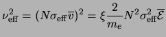
Since
![]()
![]()
![]() , where
, where
![]() is the mean electron (drift)
velocity, we define the electron mobility,
is the mean electron (drift)
velocity, we define the electron mobility,
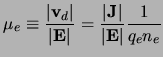
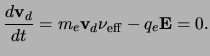
In addition, we define an effective electron-neutral
collision frequency
![]() . Assuming no
electron-electron or electron-ion (``Coulomb'')
collisions,2.2 the force
balance resulting in the net drift velocity
. Assuming no
electron-electron or electron-ion (``Coulomb'')
collisions,2.2 the force
balance resulting in the net drift velocity
![]() is the requirement
that
is the requirement
that
| (2.4) |
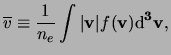
In this way we may relate macroscopic observables to the fundamental
calculable parameter
![]() and the electron distribution
function
and the electron distribution
function ![]() .
The latter, while conceptually fundamental, is not easily calculable from fundamental principles nor is it easily measureable;
however, many macroscopic measurements may shed light on it.
.
The latter, while conceptually fundamental, is not easily calculable from fundamental principles nor is it easily measureable;
however, many macroscopic measurements may shed light on it.
Lastly, as a redundant parameter, the mean free path
![]() may be
defined by
may be
defined by
It remains to justify the assumption of a small drift velocity
![]() in
equation (2.5). In addition, we derive herein a fundamental scaling
law and the time scale over which the electron distribution
function
thermalizes.2.3 Both in the
following and preceding discussions, we ignore the weak velocity
dependence of the scattering cross section, in order easily to deduce
some approximate behaviors.
in
equation (2.5). In addition, we derive herein a fundamental scaling
law and the time scale over which the electron distribution
function
thermalizes.2.3 Both in the
following and preceding discussions, we ignore the weak velocity
dependence of the scattering cross section, in order easily to deduce
some approximate behaviors.
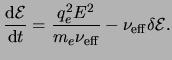
For an electron having an energy
![]() ,
a fraction
,
a fraction ![]() of its energy is lost per effective collision.
The rate of energy gain by the electron is thus the difference between
the collision term
of its energy is lost per effective collision.
The rate of energy gain by the electron is thus the difference between
the collision term
![]() and that due to the
electric field,
and that due to the
electric field,
![]() , as long as
, as long as
![]() . This
condition remains to be justified below in the context of the following discussion for
. This
condition remains to be justified below in the context of the following discussion for
![]()
![]() 3 eV; however, if elastic collisions dominate the effective collision term,
3 eV; however, if elastic collisions dominate the effective collision term,
![]() for air
[e.g., Goldstein, 1980, p. 118]. Using
(2.1) and (2.3) for
for air
[e.g., Goldstein, 1980, p. 118]. Using
(2.1) and (2.3) for
![]() we have
we have
Immediately apparent is the timescale

Equation (2.10) exhibits a key feature of electric discharges in a
weakly ionized gas. Many discharge behaviors scale linearly as
![]() , or for stronger fields as some other function of
, or for stronger fields as some other function of ![]() . As a result,
processes occurring in the relatively dilute upper atmosphere may be
studied experimentally on smaller spatial scales by using stronger electric
fields at atmospheric pressure.
. As a result,
processes occurring in the relatively dilute upper atmosphere may be
studied experimentally on smaller spatial scales by using stronger electric
fields at atmospheric pressure.
For a Maxwellian distribution,

To check whether
![]() , we use (2.1) and
(2.3) to find
, we use (2.1) and
(2.3) to find
![]() . With (2.11),
(2.10) gives
. With (2.11),
(2.10) gives
 |
(2.13) |
Referencing Figure 1.1 again and using ![]()
![]()
![]() , we see
that with
, we see
that with ![]()
![]()
![]() the thermalization time
the thermalization time
![]() is
is
![]() 10
10 ![]() s at 90 km and much faster at lower altitudes. These
simple considerations suggest that during heating driven at 90 km
altitude by a
s at 90 km and much faster at lower altitudes. These
simple considerations suggest that during heating driven at 90 km
altitude by a ![]() 20 kHz electromagnetic pulse, the electron energy
distribution is
maintained essentially in equilibrium. However, at lower values of
20 kHz electromagnetic pulse, the electron energy
distribution is
maintained essentially in equilibrium. However, at lower values of
![]() and
and ![]() ,
,
![]() increases and may become slow
compared with the electric field variation. This issue has been
explored in detail and is discussed in Section 2.2.1.
Using a detailed model for the electron distribution
function, Taranenko et al. [1993a] found that an
equilibrium mean energy of
increases and may become slow
compared with the electric field variation. This issue has been
explored in detail and is discussed in Section 2.2.1.
Using a detailed model for the electron distribution
function, Taranenko et al. [1993a] found that an
equilibrium mean energy of ![]() 4.3 eV was reached in 10
4.3 eV was reached in 10 ![]() s for
an electric field of 10
s for
an electric field of 10
![]() at 90 km altitude.
at 90 km altitude.
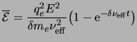
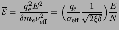
Lastly, we note that a pleasing form of (2.10) is obtained using (2.6):

As a result, on short timescales, ions and neutrals are in a separate
thermal equilibrium from that of the electrons. The value
![]() remains very small as long as only
elastic collisions are accessible (
remains very small as long as only
elastic collisions are accessible (
![]()
![]() 1.8 eV), and the
direct proportionality between
1.8 eV), and the
direct proportionality between
![]() and
and ![]() from equation (2.10) remains
strictly true. However, for
from equation (2.10) remains
strictly true. However, for ![]()
![]()
![]()
![]()
![]() eV inelastic
processes with N
eV inelastic
processes with N![]() become available, and for average energy
become available, and for average energy
![]()
![]() 0.5 eV,
electrons lose
0.5 eV,
electrons lose ![]() 90% of the energy gained from heating by an
electric field to the excitation of molecular vibrations
[Bazelyan and Raizer, 1998, p. 22]. For
90% of the energy gained from heating by an
electric field to the excitation of molecular vibrations
[Bazelyan and Raizer, 1998, p. 22]. For
![]() in the range of 10 to
15 eV, electronic levels, which are largely responsible for optical
emissions, are excited, and above 12.2 eV for O
in the range of 10 to
15 eV, electronic levels, which are largely responsible for optical
emissions, are excited, and above 12.2 eV for O![]() and 15.6 eV for
N
and 15.6 eV for
N![]() , molecular ionization is possible. At these energies inelastic
energy losses dominate over elastic ones and
, molecular ionization is possible. At these energies inelastic
energy losses dominate over elastic ones and ![]() tends to 1,
making modeling based on the simple considerations used in Section 2.1.2
essentially invalid.
tends to 1,
making modeling based on the simple considerations used in Section 2.1.2
essentially invalid.
Even for low enough electric fields such that the electron
distribution function
![]() remains
highly isotropic (
remains
highly isotropic (
![]()
![]()
![]() ), an applied electric field can
cause the shape of
), an applied electric field can
cause the shape of ![]() to depart significantly from a Maxwellian.
Because slower electrons participate only in elastic
collisions (with inefficient energy transfer to
neutrals) while energetic electrons may lose energy (or be attached)
in inelastic processes, the high-speed end of the distribution can be
greatly diminished as compared with a Maxwellian
[Chapman, 1980, p. 124]. The resulting
so-called Druyvesteyn
distribution, in which
to depart significantly from a Maxwellian.
Because slower electrons participate only in elastic
collisions (with inefficient energy transfer to
neutrals) while energetic electrons may lose energy (or be attached)
in inelastic processes, the high-speed end of the distribution can be
greatly diminished as compared with a Maxwellian
[Chapman, 1980, p. 124]. The resulting
so-called Druyvesteyn
distribution, in which
![]() rather than the
Maxwellian form of
rather than the
Maxwellian form of
![]() , has a steeper ``tail''
and has been often used in glow discharge studies [Meek and Craggs, 1978, p.
110]. However, a detailed calculation of the
distribution function from the Boltzmann equation
which takes into account an appropriate set of inelastic collisions
may result in a slightly more complex and structured distribution, for
instance that calculated by Taranenko et al. [1993a].
, has a steeper ``tail''
and has been often used in glow discharge studies [Meek and Craggs, 1978, p.
110]. However, a detailed calculation of the
distribution function from the Boltzmann equation
which takes into account an appropriate set of inelastic collisions
may result in a slightly more complex and structured distribution, for
instance that calculated by Taranenko et al. [1993a].
The dominant inelastic processes for energized electrons in weakly
ionized air are ionization and electronic excitation of neutrals, as
already mentioned above, and electron attachment to neutrals. As a
result of the third classical mechanics fact listed above,
electrons cannot combine with electronegative species such as O![]() or
positive ions in a two-body collision. As a result, in order to
recombine, cold electrons must undergo a three body
collision such as
or
positive ions in a two-body collision. As a result, in order to
recombine, cold electrons must undergo a three body
collision such as
In accordance with equation (2.10), the rate coefficients
![]() and
and
![]() for dissociative attachment and molecular ionization in an
electrically heated ionized gas scale as a function of
for dissociative attachment and molecular ionization in an
electrically heated ionized gas scale as a function of ![]() . The
electric field at which
. The
electric field at which
![]() surpasses
surpasses
![]() is known as the
conventional breakdown electric field
and denoted
is known as the
conventional breakdown electric field
and denoted ![]() ; it follows that
; it follows that
![]() is proportional
to
is proportional
to ![]() . In a
steady electric field above this threshold,
. In a
steady electric field above this threshold,
![]() and, since the ionization rate is proportional to the electron
density,
and, since the ionization rate is proportional to the electron
density, ![]() tends to increase exponentially. This electron
avalanche process was first described by J. Townsend in 1910
[reprinted in Rees, 1973], and is applicable to all of the high
altitude discharges modeled in this work. Wilson [1925] realized
that at some altitude
tends to increase exponentially. This electron
avalanche process was first described by J. Townsend in 1910
[reprinted in Rees, 1973], and is applicable to all of the high
altitude discharges modeled in this work. Wilson [1925] realized
that at some altitude
![]() would be less than the electric field due
to the charge configuration in a thundercloud, as shown in
Figure 2.1. He thus predicted an electrical
breakdown and ensuing optical emissions.
would be less than the electric field due
to the charge configuration in a thundercloud, as shown in
Figure 2.1. He thus predicted an electrical
breakdown and ensuing optical emissions.
At much higher electric fields or over long distances ![]() and high
neutral densities such that
and high
neutral densities such that
![]() m
m![]() , air
breakdown may occur instead in the form of (corona) streamers
[Bazelyan and Raizer, 1998, p. 11] or for distances and durations adequate to
significantly heat the neutral gas, in the form of leaders
[Bazelyan and Raizer, 1998]. Streamers are ionization waves which can
propagate as narrow channels through regions where
, air
breakdown may occur instead in the form of (corona) streamers
[Bazelyan and Raizer, 1998, p. 11] or for distances and durations adequate to
significantly heat the neutral gas, in the form of leaders
[Bazelyan and Raizer, 1998]. Streamers are ionization waves which can
propagate as narrow channels through regions where ![]()
![]()
![]() . This
self-propagation is due to highly nonuniform electric fields which
result from significant
. This
self-propagation is due to highly nonuniform electric fields which
result from significant
![]() , or space charge. Streamer
breakdown is not addressed in any detail in this work, but
Section 2.3 provides references to recent overviews and
to studies relating to sprites. Nevertheless, the issue of streamer
initiation
is addressed in the context of the observations presented in
subsequent sections.
, or space charge. Streamer
breakdown is not addressed in any detail in this work, but
Section 2.3 provides references to recent overviews and
to studies relating to sprites. Nevertheless, the issue of streamer
initiation
is addressed in the context of the observations presented in
subsequent sections.
The requirements for streamer initiation have mostly been discussed in the context of spark-gap experiments. For instance, Raizer et al. [1998] and Bazelyan and Raizer [1998, p. 77] describe the critical number of avalanching electrons and a critical (minimum) radius of the avalanche region needed to transition from an avalanche to a streamer. Such considerations are appropriate for an avalanche starting from a narrow point and expanding in a gas of uniform density. In the case of sprites, streamers may sometimes form at the boundary of very large regions of enhanced ionization (Sections 2.5.1 and 5.1). Raizer et al. [1998] suggest that streamers in sprites are initiated by patches of electron temperature and density perturbations caused by the interference pattern from radiation due to complex horizontal intracloud lightning channels. An observed spatial association between a bulk discharge in the lower ionosphere and the formation of streamer channels is discussed in Section 5.1, and is not consistent with the proposal of Raizer et al. [1998].
![\includegraphics[]{figures/breakdownThresholds.eps}](img147.png) |
Figure 2.1 shows electric field thresholds required
for air breakdown as a function of altitude. Conventional breakdown
occurs at ![]() 32
32
![]() at ground level and follows the neutral
density to
at ground level and follows the neutral
density to ![]() 2
2
![]() at 70 km and
at 70 km and ![]() 8
8
![]() at 90 km altitude.
Once a streamer is initiated, it may propagate in electric fields lower
than
at 90 km altitude.
Once a streamer is initiated, it may propagate in electric fields lower
than ![]() . As shown, positively charged streamers, which propagate
parallel to the electric field, have a lower propagation threshold
than negatively charged (antiparallel to
. As shown, positively charged streamers, which propagate
parallel to the electric field, have a lower propagation threshold
than negatively charged (antiparallel to ![]() ) ones. The electric
field threshold for runaway avalanche varies between the
``relativistic'' and ``thermal'' limits, and depends on the energy of
available high-energy electrons. Above the relativistic runaway
threshold, electrons with
) ones. The electric
field threshold for runaway avalanche varies between the
``relativistic'' and ``thermal'' limits, and depends on the energy of
available high-energy electrons. Above the relativistic runaway
threshold, electrons with
![]() MeV do not thermalize
because the electric force outweighs that due to
collisions. At the thermal runaway threshold,
this is true for electrons with
MeV do not thermalize
because the electric force outweighs that due to
collisions. At the thermal runaway threshold,
this is true for electrons with
![]() eV, and above this
threshold, it is true for all electrons. At tropospheric pressures
streamers may develop into leaders, which can propagate in even lower
electric fields than streamers can, due to thermal ionization of the
neutral gas; lightning is an example. This leader development is seen
to occur in electric fields greater than 1 kV/cm [Bazelyan and Raizer, 1998, p. 256]. This value does not scale simply with neutral
density and leaders are not thought to occur at high altitudes
[Pasko et al., 1998a].
eV, and above this
threshold, it is true for all electrons. At tropospheric pressures
streamers may develop into leaders, which can propagate in even lower
electric fields than streamers can, due to thermal ionization of the
neutral gas; lightning is an example. This leader development is seen
to occur in electric fields greater than 1 kV/cm [Bazelyan and Raizer, 1998, p. 256]. This value does not scale simply with neutral
density and leaders are not thought to occur at high altitudes
[Pasko et al., 1998a].
Also shown in Figure 2.1 is the electric field
magnitude that would be observed in free space due to a charge of
200 C placed at 10 km altitude above a conducting ground. The field
drops off with altitude ![]() as
as ![]()
![]() due to the dipole resulting
from the single image
charge. When combined with the electric relaxation times shown in
Figure 1.1 and discussed in Section 1.3, these
considerations point to three likely scenarios for breakdown in the
mesosphere and lower ionosphere. Transient electric
fields following large charge redistributions (
due to the dipole resulting
from the single image
charge. When combined with the electric relaxation times shown in
Figure 1.1 and discussed in Section 1.3, these
considerations point to three likely scenarios for breakdown in the
mesosphere and lower ionosphere. Transient electric
fields following large charge redistributions (![]() 1000
1000
![]() ) in clouds
may
) in clouds
may
 |
|||
 |

![\includegraphics[]{figures/absorption.eps}](img162.png) |
The value
![]() is plotted in Figure 2.2 using
values of
is plotted in Figure 2.2 using
values of
![]() both under ambient electric field and at
both under ambient electric field and at
![]() (see Figure 1.1 on page
(see Figure 1.1 on page ![]() ). It can be seen that wave energy in the
VLF frequency range, where the spectrum of lightning peaks, is largely
absorbed over a very narrow altitude range. For low wave electric
fields, this altitude is at 80 to 84 km, while for wave electric fields
strong enough to cause a considerable ionization (
). It can be seen that wave energy in the
VLF frequency range, where the spectrum of lightning peaks, is largely
absorbed over a very narrow altitude range. For low wave electric
fields, this altitude is at 80 to 84 km, while for wave electric fields
strong enough to cause a considerable ionization (
![]() ), the
altitude is near 87 to 90 km.
), the
altitude is near 87 to 90 km.
These conclusions take into account collisions not considered in the
discussion on page ![]() (Section 1.3), but still ignore the Earth's
magnetic field. Inan [1990] discusses
reflection and absorption of the ordinary and extraordinary wave modes
using the index of refraction given in a full magnetoionic treatment
[e.g., Budden, 1985].
(Section 1.3), but still ignore the Earth's
magnetic field. Inan [1990] discusses
reflection and absorption of the ordinary and extraordinary wave modes
using the index of refraction given in a full magnetoionic treatment
[e.g., Budden, 1985].