5.3 Exponential optical decay and steady electric fields

Several criteria used for the identification of elves in narrow field-of-view photometers are discussed in Chapter 4. One additional criterion not mentioned there is the fast relaxation time scale ($<$100 $\mu$s) which is often a characteristic of optical pulses due to elves. Such fast relaxation is not typical for scattered light from lightning [Thomason and Krider, 1982; Guo and Krider, 1982], and observations outlined below show that it is also generally not observed for sprites.

On the night of 19 July 1998 a large mesoscale convective system over northwestern Mexico produced exceptionally bright sprites. Measurements were made from Langmuir Laboratory using the Fly's Eye camera, optical array, and VLF receiver, as well as an image-intensified telescopic video system described by Gerken et al. [2000]. In addition, many sprites were bright enough to be visible to the unaided and unadapted eye.

Determination of total sprite luminosity lifetimes has generally been challenging [Winckler et al., 1996; Rairden and Mende, 1995]. Video recordings give generally poor time resolution and some systems, such as the image intensifier of the Fly's Eye video, exhibit a phosphor persistence following intensely bright signals. This ``afterglow'' may last for several frames, making the instrument unreliable for quantifying long sprite durations. On the other hand, photometers designed with high time resolution are not optimized for the measurement of slowly varying, weak signals, especially in the near infrared region of the spectrum [Winckler et al., 1996]. In the Fly's Eye photometers, the slow glow of sprites often appears to decay gradually into the background photometer signal level. Extra bright sprites facilitate the measurement of these longer timescales using the Fly's Eye.

Sprites are known sometimes to occur well after (up to tens of milliseconds) an associated lightning return stroke [Bell et al., 1998]. It has been proposed that this property may be due to slowly-varying currents, possibly undetectable by ELF radio measurements, which may be flowing along the ionized return stroke channel or possibly horizontally within the thundercloud [Cummer and Stanley, 1999; Bell et al., 1998; Cummer et al., 1998b]. In some cases, a series of (positive) cloud-to-ground discharges may occur sequentially over a large horizontal distance within a fraction of a second (spider lightning), suggesting the existence of an expansive travelling network of intracloud currents [Lyons, 1996]. These events are typically accompanied by a series of sprites mirroring the propagation of the lightning below (``dancing sprites''). In such cases several sprites can occur with continuous luminosity over a large fraction of a second and may appear to be associated with several lightning strokes. This paradigm was typical for the sprites observed on 19 July 1998.

In the following sections, several notable features of sprites are discussed in the context of the observations carried out on 19 July 1998. The extra signal available on this night may have highlighted some hard-to-observe but common features of sprites, or the observations may correspond only to the special case of unusually intense ionization and emissions. Several studies have suggested that the degree of ionization in sprites can vary greatly and somewhat independently of the intensity of luminous emissions [Armstrong et al., 1998b; Armstrong et al., 2000; Heavner et al., 1998].

5.3.1 Timescales in sprite photometry

Figure 5.15 shows a sample photometric record of a bright sprite, and illustrates the existence of more than one time scale in sprites. The inset image shows an intense sprite halo and bright patches near its lower boundary at $\sim$75 km which appear to have initiated downward streamers in a manner similar to that described by Stanley et al. [1999]. This event is accompanied by the photometric signature of elves (Section 4.1) in the full array of photometers (not shown). In photometer 4 (shown) the initial optical pulse due to elves becomes very bright and is protracted for $>$2 ms. This brightness is likely to be due to the sprite halo evident in the video image. Approximately 6 ms after the event onset a pulse with characteristic rise and fall times both of $\sim$2 ms appears and then relaxes into $>$50 ms of less intense glow.

Figure 5.15: Photometric features of a bright sprite. The signal from photometer 4 is shown for part of an event at 04:38:27 UT on 19 July 1998. This sprite occurred 0.5 s after a series of intense sprites associated with a series of positive cloud-to-ground lightning discharges. The inset shows a video field of the sprite from the Fly's Eye camera, superposed by a box showing the approximate field-of-view of the photometer and a scale showing altitudes overlying a causative CG.

This example highlights several features of sprites which were frequently observed on 19 July 1998 and in the course of the annual sprite campaigns conducted by the author. Many events exhibit a bright peak which is often only a few ms in duration and tends to grow and decay with similar timescales. In addition, overall photometric durations much larger than 10 ms were found to be normal on this day, in contrast to the observations of Winckler et al. [1996].

Cummer and Stanley [1999] found that the peak in optical intensity of sprites occurred after the propagation of streamers to their lowest altitudes was complete. The same phenomenology is observed for the event shown in Figure 5.2 and may be analogous to the luminous return stroke of lightning following the connection of a leader channel to ground. In this analogy, the slower sprite glow evident in Figure 5.15 may correspond to lesser excitation of the channel during the analogue of the continuing current phase in lightning.

5.3.2 Observations of exponential optical decay

Measurements from the Fly's Eye's video camera, ELF/VLF sferic receiver, and three photometers, as well as from an ultra low frequency (ULF, $<$30 Hz) search coil, are shown in Figures 5.16 and 5.17.

Figure 5.16: Slow sprite development and ULF currents. The ULF magnetic field is obtained by integrating in time data from a magnetic loop receiver. ULF data were data provided by Martin Füllekrug. According to NLDN, the two lightning discharges were 31 km apart.

Figure 5.17: Sprite preceding cloud-to-ground lightning. A close-up of Figure 5.16.

Several notable features are apparent in the event shown in Figure 5.16. Two cloud-to-ground discharges cause sprites exhibiting both short, bright features and a longer dimmer luminosity which is not well resolved by the photometers. It is likely that this sprite sustained some luminosity during the entire time between the two lightning discharges. The ULF magnetic field indicates the existence of a vertical current flowing continuously for $>$140 ms during this period. Figure 5.17 shows the unusual fact that the brightening of the sprite in photometer 11 appears to anticipate the onset of the second cloud-to-ground discharge.

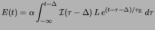
The dashed lines superposed on the photometer traces in Figure 5.17 show curves of the form

$$y(t)=C+Ae^{-t/\tau}$$ (5.1)

fit to the data by choosing values of $C$, $A$, and $\tau$. The decay of bright optical peaks in sprites is found in a large number of cases to closely follow the exponential form in (5.1) over several time constants $\tau$, although the value of $\tau$ varies considerably between different optical peaks. This rather remarkable feature of sprite optical decay has not previously been reported.

An electric field imposed on a conductive medium by a rapid rearrangement of charges is expected to decay exponentially in time (see Section 1.3, page ). Indeed, the typical timescales $\tau$ for the observed decay are comparable to expected electric relaxation times $\index{electric field!relaxation time ($\tau_{\rm E}$)}\ensuremath{\tau_{\rm E}}=\ensuremath{\epsilon_{}}/\sigma$ at the observed altitudes. However, according to Figure 2.4 on page  the optical emissions should not relax exponentially in such a case because of their highly nonlinear dependence on the electric field strength.

On the other hand, the observed exponential relaxation would be obtained if we adopt the ad hoc assumption that the electric field remains constant in time. Such an assumption was first proposed in March 1999 [Victor Pasko, private communication].

For an altitude where quenching is insignificant and with the assumptions used for equation (2.18), the optical emission rate is

$$A_k n_k \simeq \nu_k(E)\ensuremath{n_{e}}(t),$$ (5.2)

where in this case $\nu_k$ for ${\rm N}_2(1{\rm P})$ is effectively equal to $\nu_{_{\ensuremath{{{\rm B}^3\Pi_{\rm g}}}}}$$+$ $\nu_{_{\ensuremath{{{\rm C}^3\Pi_{\rm u}}}}}$ due to cascading. That is, the emission rate is the product of the electron density and a nonlinear function of the electric field, $E$. However, for $E$=$E_$=constant, $A_k n_k$$\simeq$ $\nu_k(E_)\ensuremath{n_{e}}(t)$ and we have from equation (2.15),

$$\ensuremath{n_{e}}=\ensuremath{n_{e}}\Big\vert_{t=0} e^{[\ensuremath{\nu_{\rm i}}(E_)-\ensuremath{\nu_{\rm a}}(E_)]t},$$ (5.3)

where $\ensuremath{\nu_{\rm i}}-\ensuremath{\nu_{\rm a}}$ is shown in Figure 2.4 and is also constant in time for $E=E_$. For $E_<\ensuremath{E_{k}}$ in a sprite, this condition would produce an exponential optical relaxation.

It may be cautioned that a wide variety of physical systems may be well approximated by exponential behavior, sometimes due to statistical or geometric reasons rather than those relating to local physics. For instance, in the case of elves the temporal structure of optical emissions is locally determined by temporal properties of the causative lightning pulse, and at a ground observer site is determined largely by geometrical considerations. These geometrical effects can lead to an apparently closely-exponential relaxation of luminosity from the ``back'' part of elves both in theory and observations for the case of a photometer with a field-of-view as large as that of P11 in the Fly's Eye.

Nevertheless, the exponential decay feature is found in a majority of the bright sprites observed between 04:00 and 06:00 UT on 19 July 1998 and often with a more exact fit than the cases shown in Figure 5.17. Figure 5.18 shows values of the relaxation time constant $\tau$ determined for peaks observed in 27 events exhibiting good to excellent closeness of fit between equation (5.1) and the data in narrow field-of-view photometers 1 to 9 (red filter) and 10 (blue filter). The altitudes corresponding to the narrow fields-of-view for these observations were primarily in the range 60 km to 85 km, with considerable uncertainty ($\pm12$ km) based on the possible range to the sprites, as explained on page  (Section 4.1.4).

Figure 5.18: Exponential decay times in sprites. Values shown as $\times$'s and $\circ$'s are from fits giving $R>0.7$ using data from one or more photometers in each of 27 sprite events. The *'s show the result of fits to photometric signatures of elves.

The curve fitting is done by a nonlinear least squares algorithm for periods chosen by hand to correspond well to a decaying exponential form. In some cases the initial period following a bright peak relaxes faster than the exponential fit, and not all of it is included. Instead, whenever possible, the fit period includes many times the duration of $\tau$ so as to appropriately fix the value of $C$ in equation (5.1) to the background luminosity. The quality, or closeness, of fit is then assessed by comparing the values of $\log({y-C})$ from data and fit using the linear correlation parameter $R$ given by Bevington and Robinson [1992, p. 199].

Also shown for reference are some time constants determined with the same algorithm and associated with optical pulses from the same storm but which were determined to be due to elves. The apparent close fit in these cases, however, is less significant since the parameter $\tau$ is barely resolved by the sample period of the photometer. Nevertheless, the values of $\tau$ given for elves in Figure 5.18 do give an indication of the time scales for the optical signals due to elves viewed with a narrow field-of-view. The sample period of the data is shown by a dashed vertical line.

It is apparent that while the instrument and the fitting method are capable of resolving decay constants well below 100 $\mu$s, and while the measured variation in $\tau$ extends over nearly two orders of magnitude for sprites, a lower limit of $\sim$200 $\mu$s exists among the observed sprite cases.

Two more dashed vertical lines show the fastest rate constant expected at two different altitudes for $\ensuremath{n_{e}}^{-1}(\partial\ensuremath{n_{e}}/\partial t)$ in the region where dissociative attachment dominates over ionization. As shown in Figure 2.4 on page , this rate $\ensuremath{\tau_{{\rm a}}^{{\rm min}}}$ is reached at $E\simeq0.8\ensuremath{E_{k}}$ and is also the fastest optical relaxation that is predicted for a constant electric field, according to equation (5.2). Figure 5.19 reproduces some time scales previously shown in Figure 1.1 as frequencies. Included is the variation of $\ensuremath{\tau_{{\rm a}}^{{\rm min}}}$ with altitude. The suggestion that the observed optical relaxation rate may be bounded by the maximum rate of $(\ensuremath{\nu_{\rm a}}-\ensuremath{\nu_{\rm i}})$ supports the ad hoc assumption of an essentially constant electric field during these times.

Figure 5.19: Electric relaxation and attachment time scales as a function of altitude. $\ensuremath{\tau_{{\rm a}}^{{\rm min}}}$ corresponds to the two-body dissociative attachment rate at $E$$\simeq$0.8 $\ensuremath{E_{k}}$; see Figure 2.4. The dashed line shows $\tau_{\rm E}$ for $E$$=$ $\ensuremath{E_{k}}$.

5.3.3 Steady electric currents

It is remarkable that a constant electric field should arise so frequently in a dynamically driven conducting medium. One likely scenario is the existence of a constant source current term in the troposphere over a time long compared to the local relaxation time $\index{electric field!relaxation time ($\tau_{\rm E}$)}\ensuremath{\tau_{\rm E}}$. As an example, if a thundercloud vertical charge moment change of 1000  ${\rm C\hbox{-}km}$ is required for $E$ to exceed $\ensuremath{E_{k}}$ at some altitude, then if $\index{electric field!relaxation time ($\tau_{\rm E}$)}\ensuremath{\tau_{\rm E}}$$\simeq$1 ms, a steady-state electric field of $E$$=$ $\ensuremath{E_{k}}$ could be sustained only by a current moment of 1000  ${\rm kA\hbox{-}km}$. This value is comparable to the peak current flowing in a powerful return stroke.

This relationship between current and electric field may be quantified as follows. Because of the finite atmospheric conductivity, an infinitesimal charge moment change ${\cal{I}}(\tau)L {d}\tau$ makes a contribution $dE$ to the instantaneous electric field at time $t$ which decays with time constant $\index{electric field!relaxation time ($\tau_{\rm E}$)}\ensuremath{\tau_{\rm E}}$. That is,

$$dE(t)=\alpha\; {\cal{I}}(\tau-\Delta) L e^{(t-\tau-\Delta)/\ind... ... time ($\tau_{\rm E}$)}\ensuremath{\tau_{\rm E}}}\;{d}\tau, \quad t>\tau+\Delta$$ (5.4)

for some proportionality $\alpha$, and where $\Delta$ is the speed of light propagation time. The total electric field at time $t$ is then

$$E(t)= \alpha \int_{-\infty}^{t-\Delta} {\cal{I}}(\tau-\Delta) L\... ...tric field!relaxation time ($\tau_{\rm E}$)}\ensuremath{\tau_{\rm E}}}\;{d}\tau$$ (5.5)

If the current ${\cal{I}}(\tau)$ is constant (that is, if it has been constant over time $\tau\gg\ensuremath{\epsilon_{}}/\sigma$) then the integral evaluates to

$$E(t)=E_=\alpha \; {\cal{I}}_ L\;\index{electric field!relaxatio... ...{\tau_{\rm E}}=\alpha \; {\cal{I}}_ L\frac{\ensuremath{\epsilon_{}}}{\sigma}.$$ (5.6)

Theoretical studies [e.g., Pasko et al., 1997b] suggest that sprite breakdown occurs after the integrated charge moment change surpasses a value needed to exceed the breakdown electric field. Judging from Figure 5.19 this ``integration'' may occur over times of up to $\sim$5 ms at 75 km altitude, in accordance with equation (5.5). However, once the breakdown threshold is reached the electron density may increase rapidly (for instance through streamer breakdown) on timescales much faster than $\ensuremath{\tau_{{\rm a}}^{{\rm min}}}$ and as a result the conductivity may increase drastically and the value of $\index{electric field!relaxation time ($\tau_{\rm E}$)}\ensuremath{\tau_{\rm E}}$ could be reduced to much less than that shown in Figure 5.19 for the ambient electron density. As a result, the electric field would rapidly decay (with time scale $\index{electric field!relaxation time ($\tau_{\rm E}$)}\ensuremath{\tau_{\rm E}}$) to the steady state value $E_$ given in (5.6) and thereafter the electron density and optical emissions would decay exponentially (with time scale $\ensuremath{\tau_{\rm a}}$) for any case in which $E$$<$ $\ensuremath{E_{k}}$. This entire sequence of events could occur with no temporal variation in the tropospheric source term ${\cal{I}}_ L$.

With this view, the initial non-exponential decrease following an optical peak before a closely-exponential form is observed may correspond to the establishment of a steady-state electric field $E_$. A complication to the interpretation of this sequence of events when streamers are involved is the difficulty of carrying out a theoretical calculation of the ionization level left behind a propagating streamer, where the electric field is expected to be quite low [Bazelyan and Raizer, 1998]. In light of the work of Cummer and Stanley [1999], the sequence of events described above might occur after the initial propagation of streamers is complete and may apply to the reexcitation of the remnant channels.

In any case, the measurement of exponential optical relaxation constants may constitute a significant new method for remotely sensing the local electric field within a sprite. For a given altitude observed within a narrow field-of-view, and with the assumption that $E$$<$ $0.8\ensuremath{E_{k}}$, the observed relaxation time constant $\tau$ determines $\ensuremath{\nu_{\rm i}}-\ensuremath{\nu_{\rm a}}$ which in turn prescribes $E$. In addition, according to the interpretation presented here, this observation gives non-spectral evidence of significant ionization changes. However, when taken alone it is likely not useful for measuring absolute electron densities. On the other hand, it does suggest in accordance with equation (5.3) that the free electron population likely becomes almost completely depleted in these regions where the electric field remains constant (and below $\ensuremath{E_{k}}$) for durations several times $\ensuremath{\tau_{\rm a}}$.

The ULF magnetic field data shown in Figure 5.16 indicate that an essentially time invariant continuing current in lightning is a realistic possibility, even over many milliseconds. Recent unpublished work by Steven Cummer and Martin Füllekrug has used such ULF data to infer the vertical source lightning currents with a method similar to that previously used for ELF recordings [Cummer and Inan, 2000; Cummer and Stanley, 1999; Barrington-Leigh et al., 1999a; Cummer and Inan, 1997; Cummer et al., 1998b]. The inferred vertical current moments were as high as 40  ${\rm kA\hbox{-}km}$ for 160 ms and may account for sprite breakdown in long-delayed sprites even without appealing to unmeasured horizontal charge motion, an idea which was invoked to explain previous ELF/VLF results.

On the other hand, the occurrence of a sprite just preceding the return stroke in Figure 5.17 suggests that a large (horizontal) charge motion within the cloud may have both led to a sprite and been involved in the initiation of the return stroke, indicating that horizontal currents may indeed be sufficient to initiate sprites without vertical (return stroke) charge motion. According to NLDN, the second return stroke was in a new location from the previous one. The time scale for stepped leader breakdown is $>$10 ms altogether, and $\sim$1 ms for the final leader pulse preceding the return stroke [Uman, 1987, p. 14-16], implying that the channel taken by the second return stroke in Figure 5.16 must have been developing well before the onset of the bright optical signature. An alternative interpretation for the peculiar observation of a sprite immediately preceding the second return stroke is that the timing of the sprite onset with respect to the return stroke is coincidental. However, given the 31 km proximity of the two lightning strokes as reported by NLDN, it is likely that they were closely coupled electrically through intracloud currents.

For reasons discussed previously (Section 3.1), it is difficult to determine experimentally the relative contributions of vertical and horizontal charge motions in the production of mesospheric electric fields. The results reported above give evidence of sustained source currents of one kind or another without discriminating between them.

5.3.4 Steady electric fields and streamer velocities

High speed video measurements were used to resolve the propagation velocities of ionized channels during sprite electrical breakdown [Stanley et al., 1999]. They were found to propagate at speeds of at least ${\ensuremath{2\!\times\!10^{7}}}$ m/s, in good agreement with the maximum velocity predicted by Raizer et al. [1998] for ionization waves in the form of corona streamers.

In the opposite extreme of velocity resolution, normal speed video at the high spatial resolution of a telescopic imager may be used to determine how slowly optical structures may propagate. With its 17 ms resolution and  0.7$^\circ$ vertical field-of-view corresponding to 240 pixels, the telescopic imager described by Gerken et al. [2000] may in principal resolve vertical motion as slow as ${\ensuremath{1.5\!\times\!10^{3}}}$ m/s and as fast as $\sim$10$^5$ m/s at a range of 500 km. Not surprisingly, optical structures in sprites are regularly seen which appear completely stationary on this time scale [Gerken et al., 2000]. Here we report those which appear to be coherent and in motion.

Figure: Streamer velocities. An integrated series of video fields is shown in (a) with the successive locations of some propagating features marked by $\times$'s. A number of such events from 19 July 1998 were analyzed, and the velocities of moving luminous features over time are shown in (b).

Figure a shows a portion of an integrated series of video fields from the telescopic imager. Several events from 19 July 1998 such as this one were analyzed by tracking the motion of bright features. The measured velocities are shown in Figure b as a function of time after the first appearance of luminosity in each event. In a number of events, several features were tracked and are plotted with the same color. The velocities are primarily in the range of 10$^3$ to ${\ensuremath{3\!\times\!10^{4}}}$ m/s, reflecting the resolution of the instrument, and in a number of cases luminous regions propagate steadily for 100 ms or longer.

A common approximation made in the theoretical modeling of streamers is to assume a streamer propagation velocity high compared with the mean electron drift velocity ${\bf v}_{d}$ [e.g., Dhali and Williams, 1985]. Raizer et al. [1998] conclude that streamers should not propagate when the streamer velocity approaches ${\bf v}_{d}$, and predict a lower velocity limit of $\sim10^5$ m/s. Our observations show propagation of some form, presumably in the presence of steady electric fields over tens of milliseconds, which differs from these predictions by nearly two orders of magnitude. These features, as well as static luminous regions, require further study.