3.4 The Fly's Eye

Figure 3.7: Overview of the Fly's Eye photometer array. The center image shows the photometric array, intensified CCD video camera, triggering electronics box (which includes signal filters, analog trigger circuitry, digital triggering logic, and high voltage control circuitry), and the author.

Figure 3.8: A single photometer of the Fly's Eye array. P1-P9, P11, and P13 bear red filters, while P10 and P12 bear blue ones.

The Fly's Eye photometric array was specifically designed to detect the optical emission wavelengths and space-time development predicted for elves. The spectral emissions were expected to be dominated by ${\rm N}_2(1{\rm P})$ [Taranenko et al., 1993b], especially as observed from the ground (Figure 3.6). The primary temporal and spatial requirement was to resolve an apparent motion of luminosity over $\sim$200 km in $\sim$1 ms [Inan et al., 1996c]. To resolve such an event with 10 detectors from a range of 500 km (a typical distance for demonstrated successful observation of sprites overlying distant storms) requires a temporal resolution of $\sim$50 $\mu$s and an angular resolution in at least one dimension of $\sim$2.3$^\circ$.

An elegant arrangement to achieve such a measurement would be to use one large lens to image the sky onto an array of focal plane detectors. However, because of the difficulty in obtaining an appropriately large and convex (Fresnel) lens, and moreover because of the advantage of being able to have truly contiguous and even overlapping detector fields-of-view of arbitrary shape and varying sizes, separate optics were built for each detector. Photodiodes, photomultiplier tubes (PMTs), and charge-coupled devices (CCDs) could all have met the speed criterion, but photodiodes have inferior sensitivity and the cost and time required to develop a custom CCD high-speed clocking circuit were prohibitive.

Figure 3.9: The Fly's Eye deployed at Langmuir Laboratory. The Fly's Eye (shown here with the video system removed and with fellow student Elizabeth Gerken) is mounted on a rack which contains power supplies and the control/data acquisition computer. The video recorders and the GPS receiver are located inside the laboratory.

Figure 3.7 shows a schematic overview of the Fly's Eye instrument designed and built by the author, and Figure 3.9 shows the instrument deployed at Langmuir Laboratory. Nine individually mounted photometers (P1-P9) provide the angular resolution ($\sim$2.2$^\circ$) to resolve flash features 20 km wide at a range of 500 km, and four additional photometers (P10-P13) survey larger fields-of-view. Each detector consists of a single compound lens, optical filter, and a Hamamatsu HC-124-01 or HC-125-01 PMT with built-in transimpedance preamplifier, as shown in Figure 3.8. The pointing direction of each photometer is determined by its mechanical mount, and the shape of its field-of-view is determined by a focal plane mask. The PMT photocathodes are sensitive between 185 nm and 800 nm wavelength (see PMT response curve in Figure 3.6), in and near the visible range. Two different kinds of optical filter, detailed in Figure 3.6, are used on different photometers, and may be used to determine excitation ratios, as outlined in Section 3.3.3. Empirical determination of the photometer responses and fields-of-view is discussed in Sections 3.4.1 and 3.4.2.

In addition to the thirteen amplified photometer signals, the Fly's Eye includes an Applied Geomagnetics two-axis electronic clinometer used to record automatically the viewing elevation angle, and receives one or two sferic channels from an ELF/VLF (30 Hz to 25 kHz) receiver (Figure 3.7). Using custom software developed in Visual C++, these sixteen signals (or any chosen subset) are sampled continuously in a circular buffer by two National Instruments PCI-MIO-16E-1 data acquisition boards using differential inputs in a Windows NT computer. Sample periods for each channel varied from 30 $\mu$s in 1996 to 10 $\mu$s in 1999 as the computer hardware was upgraded each year. Acquisition cycles (one per event) are started using a global positioning system (GPS) 1 Hz pulse for precise time synchronization. Trigger circuitry for several photometers and a sferic channel is used to trigger the software to save a specified portion of pre-trigger and post-trigger data from the circular buffer. In 1999 the sferic trigger circuitry included a high-pass filter and rectifier in order to respond to VLF pulses of either polarity. Typically 1 to 2 seconds of data are recorded for each trigger event. After a trigger, the data acquisition system does not record data until the next GPS second begins.

3.4.1 Pointing Calibration

The pointing direction of each photometer is mechanically fixed with respect to the Fly's Eye's base. The focal plane screen on each photocathode sets the size and shape of the field-of-view. Small adjustments can be made to its position by means of the adjustment screws holding the photomultiplier assembly (Figure 3.8).

Figure 3.10: Parallax in pointing calibrations. The blue lines terminated with $\times$'s show the locations of photometer apertures for $\phi$=0, $\theta$=0. Altered positions after a sample rotation of the Fly's Eye are shown in magenta. For nearby light sources parallax occurs due to the finite separation of the apertures.

In order to quantify the actual fields-of-view once the array was built, the photometer angular responses and fields-of-view were calibrated by scanning the Fly's Eye in azimuth and elevation past a fixed light source. Because the Fly's Eye photometers are mounted up to $>$50 cm apart from each other, parallax (i.e., the difference in the apparent direction of an object as seen from two different points) is more significant than 0.1$^\circ$ for light sources closer than $\sim$300 m. The calibration light source with small (1 cm$\times$1 cm) aperture and steady output was placed $\sim$360 cm from the Fly's Eye. Intensities in each photometer were recorded for a large number of electronically recorded elevations and at azimuths every 0.5$^\circ$. Knowledge of the precise geometry of the Fly's Eye photometers was used to correct for parallax. The position of each aperture with respect to the elevation ($\theta$) and azimuth ($\phi$) rotation axes was used to calculate, for each measurement and each photometer, the effective elevation and azimuth for a light source at infinite range. Figure 3.10 shows an example of the parallax in photometer 1 for one position of the Fly's Eye. The rotated locations $\ensuremath{\bf r_{\rm i}}'$ of the apertures were calculated in a cartesian coordinate system centered at the intersection of the rotation axes. Positions $\bf r_{\rm i}$ of the apertures for zero elevation and at a reference azimuth were measured, and $\ensuremath{\bf r_{\rm i}}'$ were calculated as

$$\ensuremath{\bf r_{\rm i}}'= \begin{pmatrix}\ensuremath{\cos{\the... ...theta}}& 0 & \ensuremath{\cos{\theta}}\end{pmatrix} \ensuremath{\bf r_{\rm i}}$$

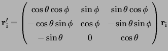
The effective azimuth $\ensuremath{\phi_{\rm eff}^i}$ and elevation $\ensuremath{\theta_{\rm eff}^i}$, corrected for parallax, are then given by

$$\cos{\ensuremath{\phi_{\rm eff}^i}} = \frac{\bf\hat{x}\cdot\ensuremath{{\bf P}_{\rm xy}(\ensuremath{\bf... ...{\bf P}_{\rm xy}(\ensuremath{\bf r_{\rm s}}-\ensuremath{\bf r_{\rm i}}')}\Vert}$$

$$\cos{\ensuremath{\theta_{\rm eff}^i}} = \frac{{\bf\hat{x}\cdot}P_{xz}(\ensuremath{\bf r_{\rm s}}-\ensurem... ...{\bf P}_{\rm xz}(\ensuremath{\bf r_{\rm s}}-\ensuremath{\bf r_{\rm i}}')}\Vert}$$

for each photometer $i$. Here $\bf r_{\rm s}$ is the position of the light source; $\bf\hat{x}$ is a unit vector pointing along the direction of $\phi=0$, $\theta=0$; $\ensuremath{{\bf P}_{\rm xy}(\bf r)}$ denotes a projection of $\bf r$ onto the plane where $\theta=0$; and $\ensuremath{{\bf P}_{\rm xz}(\bf r)}$ denotes a projection of $\bf r$ onto the plane where $\phi=0$.

Figure 3.11: Calibrated photometer fields-of-view in 1998. The data have been gridded to $0.5^\circ$$\times$$0.5^\circ$ resolution. The elevation corresponds to that read by the electronic clinometer.

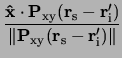
The resulting data giving measured photometric intensities at viewing directions ( $\ensuremath{\phi_{\rm eff}^i}$, $\ensuremath{\theta_{\rm eff}^i}$) were gridded for each photometer and contours of the measured sensitivity are shown in Figure 3.11. The fields-of-view do not quite correspond to the ideal design arrangement. However, once characterized, the particular field-of-view arrangement can be taken into account in detailed data analysis such as that given in Sections 4.3 and 5.1.4. Figure 3.11 shows the fields-of-view in 1998. Prior to 1998, the blue photometers P10 and P12 roughly overlaid P2 and P8, respectively, but were $\sim$3 times as large.

Figure 3.12: Cross-section of the Fly's Eye photometer responses.

Figure 3.12 shows a cross-section along the azimuth and through the peak of each photometer response in order to demonstrate the low ``cross-talk'' attained with the focal plane masks. Outside the $\sim$2$^\circ$ horizontal fields-of-view of the narrow photometers P1 to P9 the response remains below the peak response by a factor of 25 to more than 100. P4 satisfies this criterion but is highly saturated at the levels used in this calibration.

3.4.2 Intensity Calibration

Overall gains in the Hamamatsu PMT assemblies, as tested by the manufacturer, varied by two orders of magnitude from one unit to another. Values for $\alpha_{_{\rm 700 nm}}$ and $\alpha{_{\rm 400 nm}}$ were determined in accordance with equation (3.7). A calibrated Hoffman Engineering Corporation Spectral Radiance Standard with known spectrum was used as a light source, and the integral in equation (3.7) was carried out over the filter responses shown in Figure 3.6. The values for $\Omega_{\rm obs}$ were taken from the pointing calibration described above.

Surface brightnesses are subsequently expressed in kiloRayleighs (kR) at 700 nm for photometers bearing a red filter (P1 to P9, P11, and P13) and at 400 nm for those with a blue filter (P10 and P12).